Like a Bull in a China Shop… Or How to Run Neural Networks on Embedded Systems

Introduction

Connected objects are more and more present in our daily life and are bound to be unavoidable. Smart cities, autonomous cars, industrial robots, connected medical devices are only a few examples but show the large variety of domains where technology becomes more portable. Bringing computing and machine learning closer to where sensors gather data is a big challenge for embedded systems to thrive.

Different crucial issues can motivate local processing, i.e. data analysis directly inside the device:

• Data privacy concerns, especially when dealing with sensitive data, impede the data to be transmitted to third parties.
• Real time applications, for autonomous cars for instance, require immediate analysis and cannot work properly if there is a time delay to send the data elsewhere for analysis.
• Some applications need to be able to work without Internet connection.
• Bandwidth is also a great concern and local processing allows to avoid connecting to a server.
• Power is a scarce resource for embedded systems and transferring data can be very energy-costly.

However local processing, and more specifically deep learning in embedded systems, comes with a lot of hurdles. Over time networks have greatly improved in accuracy for image classification or object detection but this came at the cost of increasing computational complexity requiring ever-more GPU power and days or weeks of training.

Deep learning in embedded systems has three main challenges:

In this context, running neural networks on resource-constrained devices requires joint solutions from data engineering and data science which are sometimes called “algorithm and hardware co-design”.

The figure below, from Song Han class in Stanford on Efficient Methods and Hardware for Deep Learning, illustrates this idea.

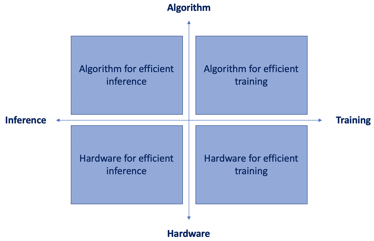Figure 1: Algorithm and Hardware co-design

In the present article we’ll discuss the algorithm part only. What are the state-of-the-art techniques to create networks that are small and fast, yet accurate?

Some techniques start from a large pre-trained network and compress it, while others directly search for simple and small network architectures.

Leveraging state of the art architectures to create smaller networks through model pruning

Model pruning

Contrary to what you may think, pruning has nothing to do with cutting trees! In machine learning, model pruning consists in removing unimportant weights in order to get a smaller and faster network. Model pruning was first introduced in 1989 by Yann Le Cun in his paper “Optimal Brain Damage”. The idea is to take a fully trained network and prune weights whose deletion will cause the least increase in the objective function. The contribution of each parameter can be approximated using the Hessian. Once unimportant weights have been removed, the smaller network can be trained once again, and the process can be iterated several times until the network has both a satisfying size and a reasonable performance.
Since then, plenty of variations of pruning techniques have been developed by researchers. In 2015, Han et al, in Learning both Weights and Connections for Efficient Neural Networks, introduced a three-step method which consists in training a neural network, then prune connections whose weight is lower than a chosen threshold and finally retrain the sparse network to learn the final weights for the remaining connections.
You may wonder, how is the pruning threshold determined? Good question! Both convolution and fully connected layers can be pruned, however experience has shown that convolution layers are more sensitive to pruning than fully connected layers. Thus, the threshold is chosen according to the sensitivity of each layer, as shown in the figure below taken from the research paper from Han et al.

Figure 2: Pruning sensitivity for CONV layer (left) and FC layer (right) of AlexNet

According to the research paper, 173 hours were necessary to retrain the pruned AlexNet on NVIDIA Titan X GPU but retraining time is not a key concern because the end goal is to make the smaller model run quickly on a resource-constrained device.
On ImageNet, the method reduced the number of parameters of AlexNet by a factor of 9x (from 61 million parameters to 6.7 million) and of VGG-16 by a factor of 13x (from 138 million parameters to 10.3 million). After pruning, the storage requirements of AlexNet and VGGNet are much lower and all weights can be stored on-chip rather than off-chip DRAM (which takes significantly more energy to access).

B. MorphNet

MorphNet, developed by AI researchers from Google in April 2017, prunes a neural network, targeting a specific resource (Floating Point Operations per Second, model size, etc) that we want to save depending on the application. MorphNet takes a pre-trained model as an input and prunes this model differently depending on the resource and the constraint defined by the user.

(pruning might have something to do with cutting trees after all)

Contrary to Neural Architecture Search (detailed in the next part), which tries to optimize every aspect of a network (filter size, width, etc), MorphNet’s task is restricted to optimizing the output width of all layers. This drastically reduces training time compared to NAS. MorphNet starts with a given seed network (Inception V2 is the seed network chosen in the research paper) and then applies two transformations to it.

First a shrinking transformation, where a sparsifying regularizer is applied on neurons, inducing some of the neurons to be zeroed out. The fact that the regularizers target neurons and not just weights is very important because pruning individual connections does not speed up computation. Indeed with this form of sparsity, all multiplication operations still need to be performed. Whereas with structured sparsity, complete lines in the weight matrix will be zeroed out allowing to skip the multiplication, as shown in the figure below:

Figure 3: Computation cost of neurons explained in a Google blog post on MorphNet: “Although the example on the left shows weight sparsity where two of the weights are 0, we still need to perform all the multiplications to evaluate this layer. However, the middle example shows structured sparsity, where all the weights in the row for neuron are 0”.

Throughout training the optimizer takes into account the resource cost when calculating gradients because a penalty is applied on the loss function:

F approximates either the number of FLOPs per inference or the model size. It implicitly depends on Θ and explicitly depends on O_1:M, the output widths of all layers.
This way, the model learns which neurons are resource-efficient and which can be removed.

The second phase is the expanding phase, where all layer sizes are expanded back, as much as the constrained resource allows, with a width multiplier w > 1. Quoting the Google blog article: « For example, if we expand by 50%, then an inefficient layer that started with 100 neurons and shrank to 10 would only expand back to 15, while an important layer that only shrank to 80 neurons might expand to 120 and have more resources with which to work. The net effect is re-allocation of computational resources from less efficient parts of the network to parts of the network where they might be more useful. »

These two steps can be repeated iteratively but a single run already brings good results according to the research paper.

How is MorphNet different from any other pruning techniques?

• MorphNet can adapt to different resource constraints while classic pruning methods focus on reducing the size of a network.
• In many pruning methods, reduced model size comes at the cost of poorer performance. That is why MorphNet has a second step and apply a width multiplier after shrinkage. Furthermore, once the new lighter structure is obtained, the original weights are not kept as is, the new network is trained from scratch instead.
• Structured sparsity greatly speeds up computations compared to other pruning methods which does not include it, such as Han et al work.

The results of the study are presented in the table below. They show that MorphNet can increase the performance of a model while maintaining the same number of FLOPS. Obviously this means that for an embedded system problem, it is possible to reduce the number of FLOPS while keeping a good accuracy.

Figure 4: Accuracy results of applying MorphNet to a variety of model architectures while maintaining FLOP cost

Rather than compressing a large network, alternative methods build instead a new neural network from scratch to get a better and smaller architecture than a human-designed one. This automated procedure is called Neural Architecture Search (NAS).

Neural Architecture Search to create resource-aware networks by design

NAS, concept and basic idea

Finding a good neural architecture is like looking for a needle in a haystack. Its is hard and very time consuming for humans. It is done via trials and errors and requires extensive domain knowledge and experience in architecture engineering to achieve state-of-the-art performances.

That is why Neural Architecture Search is a booming area of research, allowing to automate the manual task of designing the network architecture giving the best possible accuracy.

NAS involves three main concepts:

• The search space, referring to all the different possible architectures or child models that can be generated (the environment).
• The search strategy, corresponding to the method generating these architectures or child models (the policy).
• The reward-signal, which is the metric we want to optimize when generating child models.

The steps are the following:

• A recurrent neural network (RNN), called the controller, generates architectures that are defined by a string with values for the hyperparameters of the network (filter height, filter width, stride height, stride width, number of filters). RNNs are particularly suited for this task because they are able to handle variable size of input and output. In the case of NAS, the RNN takes several parameters as input but outputs only one neural architecture in the end.
• The “child networks” are trained on the real data and gives an accuracy score on a validation set
• The accuracy of the child network is used as the reward signal. The controller is updated and gives more probability to architectures that perform best. The policy gradient method (REINFORCE algorithm) is used to maximize the expected accuracy of the sampled architectures.
• The controller will learn to improve its search over time.

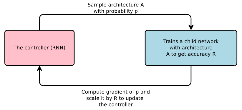
Figure 5: Overview of basic Neural Architecture Search concept

As there is an infinity of possible architectures, the search space is limited to convolutional layers in order to restrict the computational effort. This way N (N is a hyperparameter) convolution layers are stacked together to define the final network. For more details, you can read Neural architecture search with reinforcement learning from B. Zoph and Q. V. Le

B. MnasNet

It is hard to manually find a good architecture for neural networks, but it is even harder to find a simple and computationally light architecture that achieves good accuracy.

That is why Tan et al have presented MnasNet in May 2019 in their paper MnasNet: Platform-Aware Neural Architecture Search for Mobile. MnasNet has two main specificities to perform a platform-aware architecture search:

• the multi-objective function explicitly incorporates a latency metric on the reward signal.
• the search space is a “factorized hierarchical search space”, a sequence of factorized blocks, each block containing a list of layers defined by a hierarchical sub search space with different convolution operations and connections.

How is latency optimized with multi-objective function?
Considering both accuracy and latency in the optimization problem forces the search to identify a model that achieves a good trade-off between accuracy and latency. Each sampled model is trained on the target task to get its accuracy and run on real phones to get its inference latency. The reward value is then recalculated. At the end of each step, the parameters θ of the controller are updated by maximizing the expected reward. The sample-eval-update loop is repeated until it reaches the maximum number of steps or the parameters θ converge.

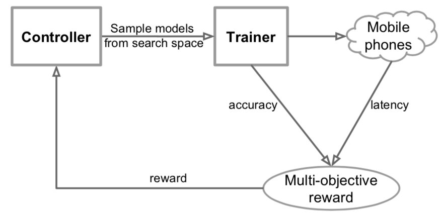
Figure 6: Overview of MnasNet concept

How is the factorized hierarchical search space defined?
In their paper, Tan and al questioned the commonly used technique that searches for the parameters of one convolution cell and then repeatedly stacks them to form the network. They show that operations like convolution greatly differ in latency depending on the concrete shapes they operate on. For instance, the first layers of CNNs usually process larger amounts of data and have higher impact on inference latency than later stages. That is why they define a new, larger search space, the “factorized hierarchical search space”. This way, different operations can be chosen at different depths of the architecture. The CNN model is partitioned into a sequence of pre-defined blocks. Similarly to classical NAS, a cell is determined and repeated N times but contrary to NAS this only constitutes one block.

Figure 7: Factorized hierarchical search space

Experiments were done on ImageNet and the real-world latency of each sampled model was measured by running it on the single-thread big CPU core of Pixel 1 phones.
The results are displayed in the table below, taken from the research paper:

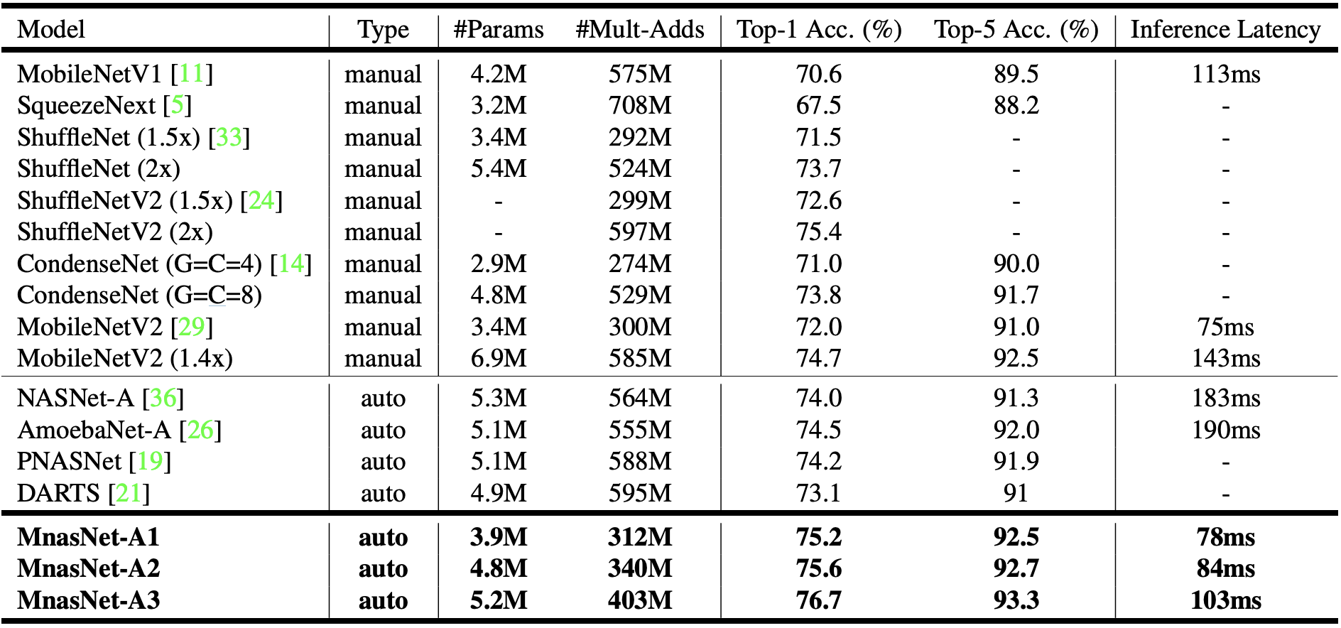
Figure 8: Performance Results on ImageNet Classification. MnasNet models are compared with both manually designed mobile models and other automated approaches – MnasNet-A1 is the baseline model;MnasNet-A2 and MnasNet-A3 are two models (for comparison) with different latency from the same architecture search experiment; #Params: number of trainable parameters; #Mult-Adds: number of multiply-add operations per image; Top-1/5 Acc.: the top-1 or top-5 accuracy on ImageNet validation set; Inference Latency is measured on the big CPU core of a Pixel 1 Phone with batch size 1.

MobileNetV2 achieves the lowest inference latency but MnasNet-A1 displays a gain of 2.5 point in top-5 accuracy for an increase of only 3ms in latency.

However, the big drawback of Neural Architecture Search, including MnasNet, is that learning the architecture requires days of GPU training. The MnasNet research paper specifies that each architecture search takes 4.5 days on 64 TPUv2 devices. Thus, MobileNetV2 still appears as the best trade-off to get low latency, good accuracy and reasonable training cost.

Conclusion

In this article we exposed different techniques to generate neural networks that are smaller and less computationally intensive in order to be able to use them on embedded systems.
Plenty of pruning methods have been developed to achieve this goal and have demonstrated good performances provided the pruned network is retrained from scratch. Neural Architecture Search is a newer area of research. These techniques display promising results in terms of accuracy for smaller networks. However, the learning process is very long and implies important GPU power because each child networks takes hours to train, making the amount of resources required prohibitive.

Sources

Efficient Methods and Hardware for Deep Learning, Stanford Lecture by Song Hal
Y. LeCun, J. S. Denker, and S. A. Solla. Optimal brain damage
Song Han, Jeff Pool, John Tran, William J. Dally. Learning both Weights and Connections for Efficient Neural Networks
B. Zoph and Q. V. Le. Neural architecture search with reinforcement learning. ICLR, 2017.
Mingxing Tan, Bo Chen, Ruoming Pang, Vijay Vasudevan, Mark Sandler, Andrew Howard, Quoc V. Le. MnasNet: Platform-Aware Neural Architecture Search for Mobile

Article écrit par Victoire de Chabalier